abdbeam

Abdbeam : composites cross section analysis

A Python package for the cross section analysis of composite material beams of any shape.

Main features

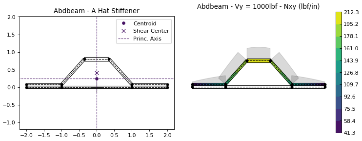
These are a few things you can do with Abdbeam:

• Use a fast thin-walled anisotropic composite beam theory including closed cells, open branches, shear connectors and booms (discrete stiffeners containing axial and torsional stiffnesses);
• Recover replacement stiffnesses (EA, EIyy, EIzz, EIyz, GJ) and/or a full 4 x 4 stiffness matrix for beams with arbitrary layups and shapes;
• Recover centroid and shear center locations;
• Obtain internal load distributions (Nx, Nxy, Mx, My, Mxy for segments; Px and Tx for booms) for a large number of cross section load cases (defined by Px, My, Mz, Tz, Vy and Vz section loads);
• Plot cross sections, their properties and internal loads.

Installing

Install using PyPI (Python package index) :

pip install abdbeam

Source and Documentation

The source code is hosted on GitHub at https://github.com/victorazzo/abdbeam and the documentation can be found at https://docs.abdbeam.org.

Dependencies

• NumPy
• Pandas
• Matplotlib

Example

Let's use Abdbeam to analyze the cross section with two closed cells below:

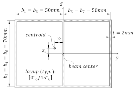
Start creating the section materials, its points and segments (we'll also calculate the section properties and request a summary at the end):

import abdbeam as ab
sc = ab.Section()
# Create a materials dictionary:
mts = dict()
mts[1] = ab.Laminate()
ply_mat = ab.PlyMaterial(0.166666, 148000, 9650, 4550, 0.3)
mts[1].ply_materials[1] = ply_mat
mts[1].plies = [[0,1]]*6 + [[45,1]]*6
# Create a points dictionary based on Y and Z point coordinates:
pts = dict()
pts[1] = ab.Point(0, -35)
pts[2] = ab.Point(-50, -35)
pts[3] = ab.Point(-50, 35)
pts[4] = ab.Point(0, 35)
pts[5] = ab.Point(50, 35)
pts[6] = ab.Point(50, -35)
# Create a segments dictionary referencing point and material ids:
sgs = dict()
sgs[1] = ab.Segment(1,2,1)
sgs[2] = ab.Segment(2,3,1)
sgs[3] = ab.Segment(3,4,1)
sgs[4] = ab.Segment(4,1,1)
sgs[5] = ab.Segment(4,5,1)
sgs[6] = ab.Segment(5,6,1)
sgs[7] = ab.Segment(6,1,1)
# Point the dictionaries to the section
sc.materials = mts
sc.points = pts
sc.segments = sgs
# Calculate and output section properties
sc.calculate_properties()
sc.summary()

Which prints:

Section Summary
===============

Number of points: 6
Number of segments: 7
Number of cells: 2

Centroid
--------
yc     = -2.67780636e-01
zc     = 0.00000000e+00

Shear Center
------------
ys     = 2.35301214e-03
zs     = -1.45758049e-03

Replacement Stiffnesses
-----------------------
EA     = 6.80329523e+07
EIyy   = 5.24834340e+10
EIzz   = 8.36408748e+10
EIyz   = 0.00000000e+00
GJ     = 1.23762317e+10
EImax  = 8.36408748e+10
EImin  = 5.24834340e+10
Angle  = 0.00000000e+00

[P_c] - Beam Stiffness Matrix at the Centroid
---------------------------------------------
[[ 6.80329523e+07  0.00000000e+00  2.46320132e+05 -1.43701515e+08]
 [ 0.00000000e+00  5.24834340e+10  0.00000000e+00  0.00000000e+00]
 [ 2.46320132e+05  0.00000000e+00  8.36408748e+10 -2.12142163e+07]
 [-1.43701515e+08  0.00000000e+00 -2.12142163e+07  1.23762317e+10]]

[W_c] - Beam Compliance Matrix at the Centroid
----------------------------------------------
[[1.50683149e-08 0.00000000e+00 1.66286490e-28 1.74959530e-10]
 [0.00000000e+00 1.90536313e-11 0.00000000e+00 0.00000000e+00]
 [1.57282135e-25 0.00000000e+00 1.19558821e-11 2.04936911e-14]
 [1.74959530e-10 0.00000000e+00 2.04936911e-14 8.28315446e-11]]

[P] - Beam Stiffness Matrix at the Origin
-----------------------------------------
[[ 6.80329523e+07  0.00000000e+00 -1.79715871e+07 -1.43701515e+08]
 [ 0.00000000e+00  5.24834340e+10  0.00000000e+00  0.00000000e+00]
 [-1.79715871e+07  0.00000000e+00  8.36456213e+10  1.72662667e+07]
 [-1.43701515e+08  0.00000000e+00  1.72662667e+07  1.23762317e+10]]

[W] - Beam Compliance Matrix at the Origin
------------------------------------------
[[1.50691722e-08 0.00000000e+00 3.20155371e-12 1.74965018e-10]
 [0.00000000e+00 1.90536313e-11 0.00000000e+00 0.00000000e+00]
 [3.20155371e-12 0.00000000e+00 1.19558821e-11 2.04936911e-14]
 [1.74965018e-10 0.00000000e+00 2.04936911e-14 8.28315446e-11]]

Now let's create two load cases (101 and 102) and calculate their internal loads:

sc.loads = dict()
sc.loads[101] = ab.Load(My=5e6)
sc.loads[102] = ab.Load(Tx=250000, Vz=5000.0)
sc.calculate_internal_loads()

Next print all internal loads (which outputs a lot of data we'll not show here):

sc.print_internal_loads()

Or access the Pandas dataframe containing these internal loads directly:

df = sc.sgs_int_lds_df

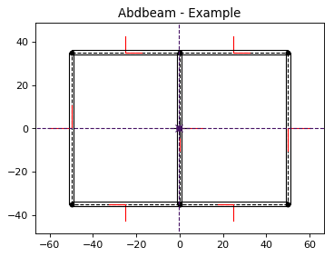
Next plot the cross section and its properties (we'll show the segment orientations, hide legends, change the centroid , shear center and principal axis colors and use a custom figure size):

ab.plot_section(sc, segment_coord=True, title='Abdbeam - Example', 
                legend=False, prop_color='#471365', figsize=(5.12, 3.84))

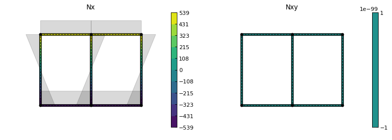
Finally, plot Nx and Nxy for load case 101 (we'll change the matplotlib contour palette, reduce the internal load diagram scale, and use a custom figure size):

ab.plot_section_loads(sc, 101, contour_color='viridis', diagram_scale=0.7, 
                      int_load_list=['Nx', 'Nxy'], figsize=(5.12, 3.84))

License

BSD-3

Contribute

Abdbeam is at its early development stages and we encourage you to pitch in and contribute on GitHub. Guidelines for contributors are in the works, so stay tuned.

Theory

For the theory behind Abdbeam, the most complete reference is:

Victorazzo DS, De Jesus A. A Kollár and Pluzsik anisotropic composite beam theory for arbitrary multicelled cross sections. Journal of Reinforced Plastics and Composites. 2016 Dec;35(23):1696-711.

These are also great references on its originating theory:

• Kollár LP, Springer GS. Mechanics of composite structures. Cambridge university press; 2003 Feb 17.
• Kollár LP and Pluzsik A. Analysis of thin-walled composite beams with arbitrary layup. J Reinf Plast Compos 2002; 21: 1423–1465.

Note: the effects of shear deformation and restrained warping are assumed negligible in Abdbeam. Check the references above for more details.