
 Repository
Current collected state Current
Observed since 20 Oct, 18:44 UTC
No superseded metadata states collected. Unchanged observations do not create new revisions.
Acute:chronic workload ratios in Python, with the diagnostics to test whether they mean anything
Acute:chronic workload ratios in Python, with the diagnostics to test whether they mean anything on your data.
The acute:chronic workload ratio divides an athlete's recent training load by their longer-term load. It is probably the most widely used number in athlete monitoring, it appears in commercial platforms and consumer running apps, and a substantial body of work argues it does not predict injury. This package computes all three published forms of it, and it ships the test its critics proposed so that anyone using it can check the question rather than take a side.
Before this package there was no Python implementation. R has two, Athlytics
on rOpenSci and ACWR on CRAN.
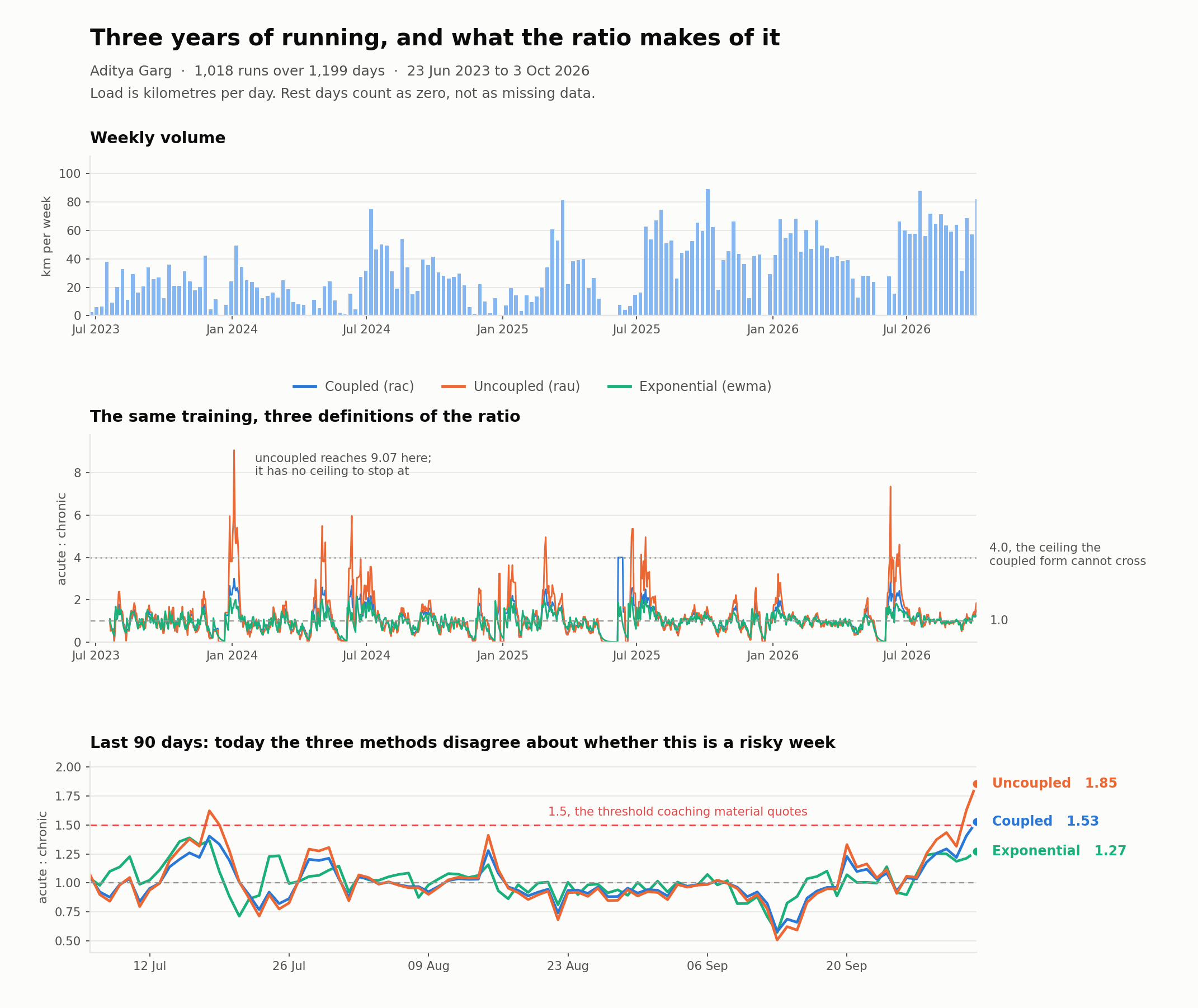
The figure above is 1,018 runs over 1,199 days. The middle panel is the same training
read three ways, and the dotted line at 4.0 is the ceiling the coupled method cannot
cross, explained below. Regenerate it with python docs/make_figure.py, which writes to out/.
Documentation: https://lombergine.github.io/acwr/
pip install acwr
Requires Python 3.10 or newer, and depends only on numpy, pandas and scipy.
From a table of activities to a ratio:
import pandas as pd
import acwr

activities = pd.DataFrame({
    "date": ["2026-01-01", "2026-01-01", "2026-01-03"],
    "load": [30.0, 20.0, 45.0],
})

load = acwr.daily_load(activities)          # continuous daily series
ratio = acwr.acwr(load, method="rac")       # the standard form
daily_load does something easy to skip and important to get right. Rolling
windows must run over a continuous daily index, so rest days are filled with
zero rather than left out. A 28 day window computed over only the days someone
trained is not a 28 day window, and that is the most common way a published
ACWR goes wrong.
Any numeric load works, since the ratio is scale free. Session RPE, minutes, distance and training stress score all behave the same way, as long as the unit is consistent.
Every number here inherits whatever is wrong with the series it was given, and training logs are wrong in a small number of reliable ways.
print(acwr.check_load(load))
Load quality: 1199 days, 662 with training, 0 error(s), 2 warning(s)
  [warn ] outlier days: 1 day(s) exceed 3 times the 95th percentile training day of 78.89, the largest being 389.4
  [warn ] break: the longest run of zero-load days is 27 days, ending 2025-06-05. The ratio on the days after it is dominated by the break rather than by the training
That output is from three years of one runner's log, and the first line is a watch left running: 389 minutes recorded for a 1.28 km run. Nothing else in the pipeline would have objected.
The checks are for a history shorter than the chronic window, a log with no training in it, negative loads, days unobserved rather than rested, outliers, suspected changes of recording unit, extreme dynamic range, long breaks, and a series that is mostly rest. Severity means something specific: an error makes the computation meaningless, a warning changes the answer without invalidating it, and a note is context for reading the output.
Outliers are judged against the 95th percentile rather than the median, and deliberately. Training load is strongly right-skewed, so a rule written against the median flags every athlete's longest run and gets ignored within a week.
Nothing is corrected automatically. Whether a thirty day gap was a planned break or a month of unsynced training is not a question a library can answer, and guessing would propagate silently into everything downstream.
acwr.acwr(load, method="rac")    # rolling average, coupled    (default)
acwr.acwr(load, method="rau")    # rolling average, uncoupled
acwr.acwr(load, method="ewma")   # exponentially weighted
They disagree, and the disagreement is the interesting part. Take four steady weeks at a load of 50, then one week at 100:
| method | ratio on the final day |
|---|---|
rac | 1.60 |
rau | 2.00 |
ewma | 1.34 |
rac is the original form, and the chronic window contains the acute window.
The hard week therefore appears in both the numerator and the denominator,
lifting the denominator from 50 to 62.5 and pulling the ratio down to 1.6. That
shared term is the mathematical coupling that Impellizzeri et al. (2020)
describe.
rau takes the chronic average over the 21 days before the acute window, so
the two halves share no data and the answer is the arithmetically clean 2.0.
ewma weights recent days more heavily, following Williams et al. (2017), on
the argument that a flat window treats a session from three weeks ago as
exactly as recent as one from yesterday.
Pass return_components=True for a frame with load, acute, chronic and
acwr, which is how you tell a high ratio caused by a hard week from one caused
by an unusually easy month.
It has a ceiling, and the ceiling is chronic / acute. Write the ratio
with sums rather than means and it becomes (chronic/acute) * (S_acute / S_chronic). The acute window sits inside the chronic window, so S_acute can
never exceed S_chronic, so the second factor never exceeds 1. At the standard
7 and 28 days the coupled ratio therefore cannot go above 4.0 no matter what an
athlete does. A value of 4.0 is not "four times the usual load", it is "every
kilometre of the last month was run in the last week". The uncoupled form has
no ceiling at all. On three years of one runner's data the coupled form capped
at 4.00 on seven days in June 2025, returning from a 27 day break, and on each
of those the uncoupled form was outright infinite, because the 21 days its
denominator covers were entirely rest. Its largest finite reading, 9.07, falls
on 4 January 2024, a day the coupled form puts at 3.01.
This ceiling is not a new observation. Wang et al. (2019) state it in a preprint, noting that the coupling "creates a theoretical maximum ACRatio of 4, regardless of the magnitude of the absolute change in workload". The passage does not appear in the published version of that work, and neither R package documents or tests the property. What this package adds is a test that holds the implementation to it.
It compresses the ratio toward 1.0 from both sides. rac reads lower than
rau on every day the ratio is above 1, and never lower on any day it is below
rac < rau works out to be the same condition as rac > 1.
Because every threshold in the literature sits above 1.0, the practical effect
is one directional: in the region anyone monitors, coupling can only
understate. On that same three years, there were 76 days the uncoupled ratio
put above 1.5 and the coupled ratio did not, and zero days the other way round.This bears on a published result. Coyne et al. (2019) compared the two forms on elite athlete data, found correlations between 0.88 and 0.99 with trivial effect sizes, and concluded there is a low risk of coupling causing spurious correlation. A high correlation between two series says nothing about whether they fall on the same side of a cut point, and the asymmetry above is what a threshold-based decision actually depends on. The two findings are compatible.
Both properties are tested rather than asserted, in
test_coupled_ratio_can_never_exceed_chronic_over_acute and
test_coupling_compresses_the_ratio_toward_one.
This is the part that does not exist elsewhere.
print(acwr.rescaling_check(load))
# ACWR vs acute load alone, n=473: Spearman 0.629 [0.564, 0.682], Pearson 0.656
That output is from the synthetic series in tests/test_diagnostics.py, not
from the three-line frame above, which is too short to produce a ratio at all.
Every sample output in this file comes from a seeded series in the test suite or
from the author's own training log, and
the worked example is runnable
end to end with a test that executes it.
The ratio is acute load divided by chronic load. When the denominator varies little next to the numerator, dividing barely changes the ordering of days and the ratio becomes a rescaled copy of the acute load. This reports how far down that road your data sits. In the limit it is exact: with a constant denominator the Spearman is 1.0, and the ratio is the numerator in different units.
result = acwr.compare_to_null(load, injured, kind="shuffle")
print(result)
(From test_random_chronic_denominator_performs_about_as_well, on synthetic
data where injury was generated from acute load alone.)
AUC, n=873 (179 events)
  real ACWR:          0.594 [0.547, 0.642]
  shuffle    null:    0.625 [0.601, 0.650]  (120 draws)
  real ratio is BELOW the null interval: the real denominator cost signal
  that a random one did not
This is the test from Impellizzeri et al. (2021). Compute the association between injury and the real ratio, then recompute it many times against ratios whose chronic denominator has been replaced by a contrivance, and compare. If a denominator can be swapped for noise without hurting the result, it was not doing any work.
Three contrivances are available. "shuffle" permutes the real chronic series,
keeping its exact distribution and destroying its timing. "normal" draws from
a distribution matched to the real chronic mean and spread. "constant" uses
the mean, which is the fixed-value version of the original test.
The output above is from the package's own test suite, on synthetic data where injury was generated from acute load alone. The real coupled ratio scores below its random-denominator null, and the reason is worth understanding: the outcome responds to acute load, and the coupled ratio divides acute load by a window containing that same load, which compresses exactly the spikes the outcome responds to. A random denominator does no such damping.
Two properties report the comparison, and they are deliberately different.
real_beats_null is one sided and true only when the real statistic exceeds
the null interval. real_outside_null is two sided. A ratio that falls below
its null has not beaten anything, and conflating those two was a bug in this
package's own first draft.
print(acwr.threshold_from_history(load))
Thresholds on this athlete's own history (rac, n=1172 usable days)
  1.5 flags 188 days (16.0%), which is this athlete's 84.0th percentile
  their own percentiles:
    50th  0.98
    75th  1.28
    90th  1.74
    95th  2.13
    99th  2.63
The same 1.5 is quoted for a marathoner in a base block and a sprinter in competition. On this runner it picks out one day in six. A coach wanting the hardest one day in twenty would need 2.13.
This is not a recommendation to personalise the threshold. A cut taken from an athlete's own distribution flags a fixed share of their days by construction, whatever their training was actually like, which is a different failure rather than a fix. The function exists to make the arbitrariness of the universal number visible.
Seven and twenty-eight days are conventional. They are not derived from anything, and papers that use them rarely say why.
print(acwr.window_sensitivity(load))
Window sensitivity at threshold 1.5 (rac, 16 window pairs)
  reference 7/28 flags 16.0% of days
  flagged fraction across pairs: 1.6% to 20.7%
  agreement with the reference: 0.02 to 0.71 (Jaccard)
This sweeps a grid of window pairs, flags the days each one puts above the threshold, and reports the Jaccard agreement between those sets of days and the set the conventional pair produces. The output above is from three years of one runner's log. No alternative pair agreed with 7/28 on more than 71 percent of flagged days, and the fraction of days flagged ranged over an order of magnitude. The window lengths moved the output more than the training did.
result.table has the full grid if you want to plot it.
The ratio asks whether this week was harder than the recent average. Foster's monotony asks whether the week was the same every day, on the argument that seven identical moderate sessions cost more to recover from than a week with a hard day and a rest day.
acwr.monotony(load)        # mean daily load over a week / its spread
acwr.strain(load)          # weekly total * monotony
acwr.weekly_blocks(load)   # the same, per calendar week, as Foster reported it
acwr.srpe_load(minutes, rpe)   # duration * rated exertion
Three details of the definition are unstable across the literature and all
three move the answer, so each is a documented parameter rather than a silent
choice. The standard deviation may be the sample one or the population one, and
for a seven day window ddof=1 gives a monotony about 7 percent lower than
ddof=0. The window may be rolling or a calendar week, and this package rolls
by default because a monitoring tool needs an answer every day. The day a week
ends on changes the blocks, and moving the boundary moves the long run from one
block to the next.
A perfectly even week has zero spread, so monotony is inf. That is the
correct answer rather than an error, and replacing it with a large finite
number would hide the thing the statistic is measuring.
The other number applied practice quotes. Gabbett (2016) reports that a rise of 15 percent or more over the preceding week is where injury risk climbs.
acwr.week_to_week_change(load)          # trailing 7 days against the 7 before
acwr.block_change(load)                 # one row per calendar week
Returned as a percentage by default, so 20.0 means a fifth more than last week.
A week following complete rest gives inf, which is arithmetically correct and
a fair summary of the metric's problem: it is least informative exactly where
the risk is most discussed.
No threshold is shipped. The 15 percent figure rests on the same literature the diagnostics below exist to let you test.
Rolling a window over a frame sorted by date instead of grouped by athlete will average one runner's Tuesday into another's Wednesday, and the result looks plausible.
acwr.by_athlete(activities, acwr.acwr, acute=7, chronic=28)
acwr.by_athlete(activities, acwr.monotony, window=7)
Takes a long frame with an athlete column, builds each athlete's daily series
separately, applies any per-athlete function, and returns a long frame.
Each athlete spans their own first to last activity by default, because padding
a late joiner back to the squad's first day invents rest days they never had.
Pass common_calendar=True when they genuinely share a season.
pip install 'acwr[plot]'
fig, (top, bottom) = acwr.plot_acwr(load, methods=("rac", "rau"))
fig, ax = acwr.plot_window_sensitivity(acwr.window_sensitivity(load))
Both return the axes they drew on and neither calls show or savefig.
Importing acwr does not require matplotlib; the two helpers import it on
first touch.
The usual plot of a workload ratio makes two mistakes, and these avoid both.
It puts load and ratio on one pair of axes with two scales, inviting a
comparison between two quantities whose relative heights mean nothing, so
plot_acwr stacks two panels with one scale each. And it shades a "sweet spot"
band behind the line, asserting exactly the thresholds this package declines to
ship, so nothing is shaded. The rule drawn at 1.0 is there because a ratio of
1.0 means this week matched the recent average, which is a fact about division.
It does not claim the ratio predicts injury. The weight of the evidence runs the other way, and the package exists partly to make that evidence easy to reproduce.
It does not claim the ratio is worthless either. The diagnostics are descriptive, they are not hypothesis tests, and a result on one dataset is a result on one dataset.
It does not model injury risk, recommend training, or output a safe range. The "sweet spot" bands that circulate in coaching material do not appear anywhere in this code, because the thresholds they rest on come from the same literature whose foundations are in dispute.
In scope: checking a training log before anything is computed from it, building the daily load series, the three ratio methods, Foster's monotony and strain, week-to-week change, per-athlete application across a squad, the diagnostics above, and plots of the result.
Not in scope, deliberately: readers for FIT, TCX and GPX files. Parsing device formats is a substantial job that existing libraries already do well, so the plan is to document how to pipe their output in rather than to re-implement them.
If you use a particular method, cite its source rather than this package alone.
Coyne, J. O. C., Nimphius, S., Newton, R. U., & Haff, G. G. (2019). Does mathematical coupling matter to the acute to chronic workload ratio? A case study from elite sport. International Journal of Sports Physiology and Performance, 14(10), 1447-1454.
Gabbett, T. J. (2016). The training-injury prevention paradox: should athletes be training smarter and harder? British Journal of Sports Medicine, 50(5), 273-280.
Foster, C. (1998). Monitoring training in athletes with reference to overtraining syndrome. Medicine & Science in Sports & Exercise, 30(7), 1164-1168.
Williams, S., West, S., Cross, M. J., & Stokes, K. A. (2017). Better way to determine the acute:chronic workload ratio? British Journal of Sports Medicine, 51(3), 209-210.
Impellizzeri, F. M., Tenan, M. S., Kempton, T., Novak, A., & Coutts, A. J. (2020). Acute:chronic workload ratio: conceptual issues and fundamental pitfalls. International Journal of Sports Physiology and Performance, 15(6), 907-913.
Wang, C., Vargas, J. T., Stokes, T., Steele, R., & Shrier, I. (2019). The acute:chronic workload ratio: challenges and prospects for improvement. arXiv:1907.05326. Published in revised form as Wang et al. (2020), Analyzing activity and injury: lessons learned from the acute:chronic workload ratio, Sports Medicine, 50(7), 1243-1254.
Impellizzeri, F. M., Woodcock, S., Coutts, A. J., Fanchini, M., McCall, A., & Vigotsky, A. D. (2021). What role do chronic workloads play in the acute to chronic workload ratio? Time to dismiss ACWR and its underlying theory. Sports Medicine, 51(3), 581-592.
Athlytics (rOpenSci) computes the coupled rolling average and an EWMA variant
in R, and reads Strava and device files, which this package does not.
ACWR (CRAN) implements all three methods in R. Neither ships a null-model
diagnostic.
Athlytics is the reference implementation, so its source was read and its
coupled rolling-average path is reproduced in this package's test suite
(test_coupled_method_matches_the_athlytics_algorithm). On identical input the
two agree to floating point. Three differences are worth knowing before
comparing outputs across the two.
The EWMA decay is parameterised differently, and the same N means different
things. Williams et al. (2017) specify lambda = 2 / (N + 1), which is what
this package does by default. Athlytics uses a half-life instead,
alpha = 1 - exp(-ln 2 / N). For N = 7 that is 0.25 against roughly 0.094, so
the half-life form decays far more slowly and a spike takes much longer to show
up. Pass decay="half_life" to match Athlytics:
acwr.acwr(load, method="ewma", decay="span")       # Williams et al. (default)
acwr.acwr(load, method="ewma", decay="half_life")  # Athlytics-compatible
Smoothing here is trailing, not centred. Athlytics smooths right-aligned and
that is correct. The first draft of this package centred the window, which meant
today's smoothed ratio depended on the next few days of training. For a tool
meant to inform a training decision that is a bug rather than a preference, and
it is now trailing by default with smooth_center=True available for
retrospective plots.
Division by a near-zero chronic load is handled differently. Athlytics
returns NA below a 0.01 floor; this package returns inf, which keeps
"trained hard off no base" distinguishable from "no data".
Two things are worth separating here, because an earlier draft of this file ran them together. Division by exactly zero on a positive numerator is impossible for both the coupled and the exponentially weighted methods, since in each the denominator includes today's load, so a positive numerator forces a positive denominator. Only the uncoupled method can do it, and it does: on 400 random series it divided by zero 2,636 times while the other two did it never.
A floor at 0.01 is a different matter and can fire on any of the three. One 0.1 km day after 27 days of rest gives a coupled acute of 0.0143 against a chronic of 0.0036, which is under the floor, and the ratio is a perfectly meaningful 4.0. Which is to say the floor is a choice about small numbers, not a guard against an impossible operation.
See CONTRIBUTING.md and CODE_OF_CONDUCT.md. Bug reports with a reproducible example are the most useful thing, and a failing test is better than a description.
Claude was used as a pair programmer throughout, and AI-USAGE.md says exactly what it did, what the author did, and the five errors the process produced along with the mechanism that caught each one.
MIT. See LICENSE.
Download counts and popularity will appear here as the collector receives them.
| Version | Published | Direct dependencies | Open version |
|---|---|---|---|
| 0.1.1 | 5 Oct 2026 | 14 |
This describes our collected data; it is not a security assessment.
Observed since 20 Oct, 18:44 UTC
No superseded metadata states collected. Unchanged observations do not create new revisions.
package:0f78e03260247fd04ad7bb184f951114b8e6c774e4a907946ee24229a860b43d