

 Repository
Current collected state Current
Observed since 20 Oct, 20:09 UTC
No superseded metadata states collected. Unchanged observations do not create new revisions.
Four-parameter semi-empirical electrochemical and thermal model of alkaline water electrolysers (AWE/AEC), with fitting tools and literature datasets.


A lightweight Python package for alkaline water electrolysis (AWE / AEC). It provides:
It is intended for system-level studies such as power-to-hydrogen plants, temperature control, lye-cooling sizing and techno-economic analysis. In these studies you need a model that is fast, robust and extrapolates sensibly in temperature.
The package was developed during a visiting PhD period (2022) at DTU Energy under the supervision of Henrik Lund Frandsen.


pip install aec-modelling            # core: numpy, scipy, pandas
pip install "aec-modelling[plot]"    # + matplotlib plotting helpers
From source, for development:
git clone https://github.com/Lingkangjin/AEC-Modelling.git
cd AEC-Modelling
uv sync --extra dev          # or: python -m pip install -e ".[dev]"
Python ≥ 3.9 is required.
import numpy as np
from aec_modelling import AECModel, datasets, fit_polarization

# 1. Fit the four parameters on a literature dataset (or your own DataFrame)
df = datasets.load("sakas")          # columns: j [mA/cm2], T [K], V [V], P [bar], w [-]
fit = fit_polarization(df)
print(fit.summary())

# 2. Use the calibrated model
cell = fit.model
cell.voltage(300, 353.15)                    # V at 300 mA/cm2, 80 °C
cell.overpotentials(np.linspace(10, 500, 50), 353.15)   # DataFrame: V_rev, V_act, V_ohm, V_cell, V_tn
cell.current_density(1.9, 353.15)            # inverse: j at 1.9 V
cell.voltage_efficiency(300, 353.15)         # V_tn / V_cell
Four-parameter AEC model fit
--------------------------------------------
 delta_l =      0.59344 +/- 0.0364     [cm]
   alpha =      0.13121 +/- 0.00803    [-]
      C1 =      -6646.3 +/- 397        [K]
      C2 =       20.816 +/- 1          [-]
--------------------------------------------
points = 40   R2 = 0.9982   RMSE = 3.6 mV
activation energy Ea = 55.3 kJ/mol
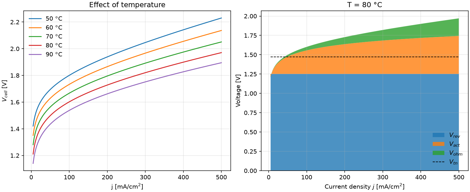
V_cell = V_rev + V_act + V_ohm

V_rev = U0(T) + RT/(2F) · ln[ (P − p_v)^1.5 / a_w ]     reversible
V_act = RT/(2·alpha·F) · ( ln j − C1/T − C2 )            activation (Tafel)
V_ohm = delta_l · j / sigma(T, w)                        ohmic
| Parameter | Unit | Physical meaning |
|---|---|---|
delta_l | cm | effective ionic path length (gap + separator + bubbles) |
alpha | – | lumped charge-transfer coefficient, which sets the Tafel slope |
C1 | K | Arrhenius slope of the exchange current density (activation energy Ea = −C1·R) |
C2 | – | Arrhenius intercept of ln i0 |
The reversible voltage, electrolyte conductivity, vapour pressure and water activity come from literature correlations that depend on temperature, pressure and KOH concentration. Only the four parameters above are fitted. The full equations are in docs/model.md.
Put your measurements in a DataFrame with one row per point:
| column | unit | |
|---|---|---|
j | mA/cm² | current density (> 0) |
T | K | cell / stack temperature |
V | V | per-cell voltage |
P | bar abs. | optional column, or pass P=... |
w | – | KOH mass fraction, optional column, or pass w=... |
import pandas as pd
from aec_modelling import fit_polarization, sample_points

df = pd.read_csv("my_test_bench.csv")          # j, T, V
fit = fit_polarization(df, P=10.0, w=0.30)

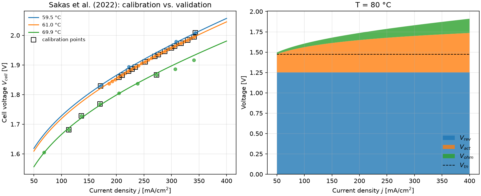
# Calibrate on 20 random points spanning 2+ temperatures and validate on the rest
calib = sample_points(df, n=20, min_temperatures=2, random_state=0)
fit = fit_polarization(calib, P=10.0, w=0.30)
print(fit.evaluate(df, by="T"))                # R2 / RMSE / MAPE per temperature

# Custom initial guess and bounds: (delta_l, alpha, C1, C2)
fit = fit_polarization(df, P=10, w=0.3, p0=(0.4, 0.13, -6330, 14),
                       bounds=((0, 0.05, -1e4, -5), (2, 1, 0, 30)))
Tips
C1 and C2 cannot be separated.activation="asinh" avoids negative activation overpotential when the data include very low current densities.
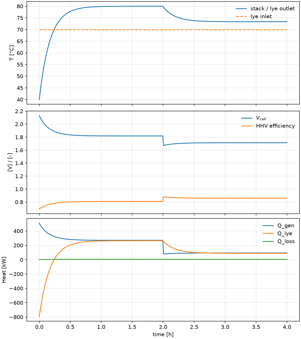
A cell releases heat when its voltage is above the thermoneutral voltage V_tn ≈ 1.48 V: Q_gen = N_cells · (V_cell − V_tn) · I. The package couples this heat source to two stack energy-balance models.
from aec_modelling import Stack, LumpedThermalModel, AxialThermalModel

stack = Stack(fit.model, n_cells=100, cell_area=2.6e4)     # area in cm2
I = stack.current(300)                                      # A at 300 mA/cm2

# 0D: well-mixed stack with lye cooling and heat losses
th = LumpedThermalModel(stack, heat_capacity=2e7, thermal_resistance=0.01)
m_lye = th.required_lye_flow(I, T_out=353.15, T_in=343.15)   # kg/s
T_ss  = th.steady_state(I, T_in=343.15, m_lye=m_lye)
t     = np.linspace(0, 4 * 3600, 400)                       # s
sim   = th.simulate(t, I=lambda t: I if t < 7200 else I/2, T_in=343.15, m_lye=m_lye, T0=313.15)

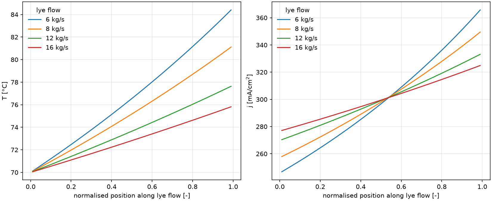
# 1D: temperature rise along the cell and the resulting current maldistribution
res = AxialThermalModel(stack, n_segments=50).solve(I, T_in=343.15, m_lye=8.0)
res.V_cell, res.T_out, res.current_maldistribution, res.profile    # profile: z, T, j, q
| 0D: warm-up and load step | 1D: profiles vs. lye flow |
|---|---|
 |  |
from aec_modelling import datasets
datasets.list_datasets()        # overview table
df = datasets.load("ulleberg")  # tidy DataFrame; metadata in df.attrs (reference, doi, notes)
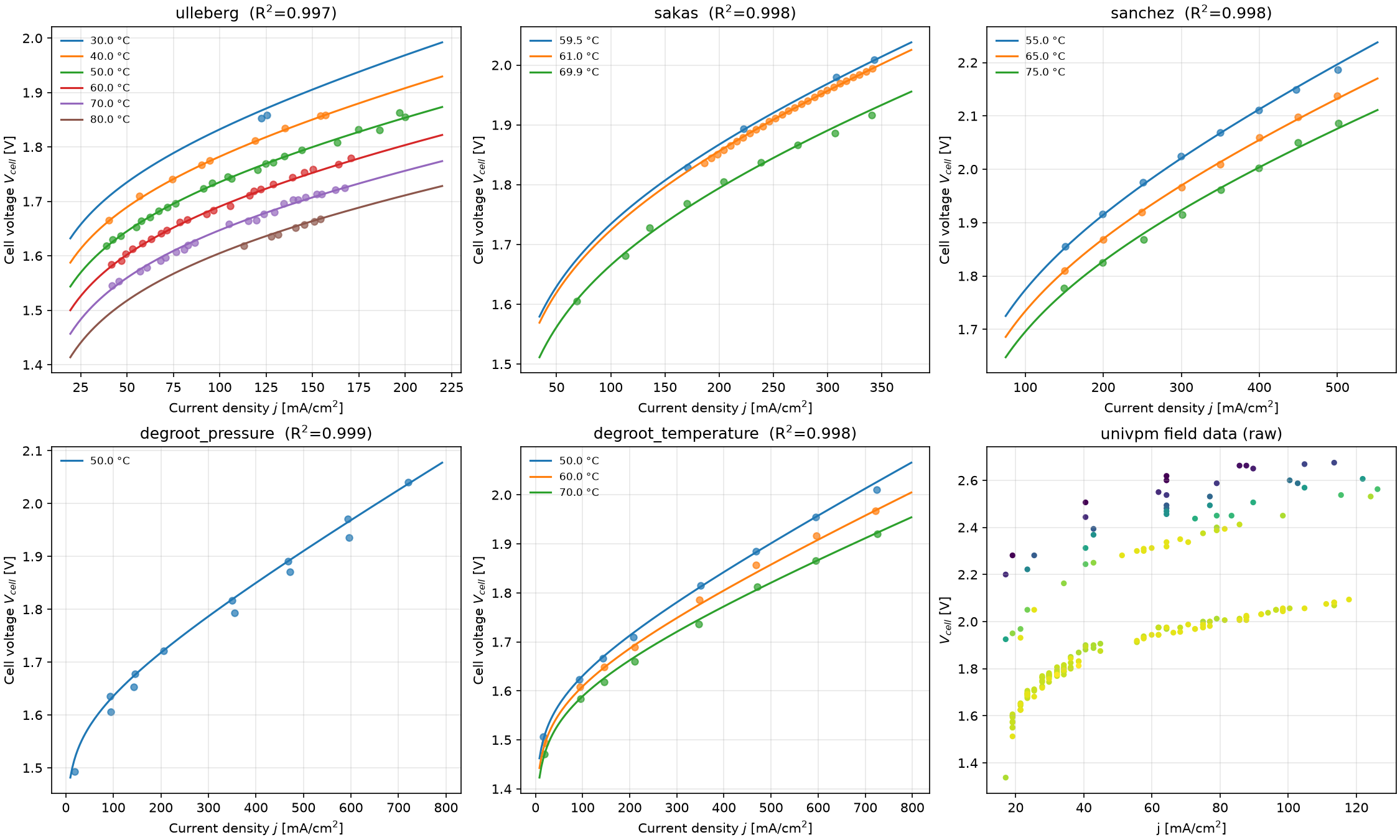
| name | source | T range | P | KOH | points | R² (all points) |
|---|---|---|---|---|---|---|
ulleberg | Ulleberg 2003, PHOEBUS 26 kW | 30–80 °C | 7 bar | 30 wt% | 86 | 0.997 |
sakas | Sakas et al. 2022, industrial 3 MW | 59–70 °C | 16 bar | 25 wt% | 40 | 0.998 |
sanchez | Sánchez et al. 2018, 15 kW stack | 55–75 °C | 7 bar | 35 wt% | 24 | 0.998 |
degroot_pressure | de Groot et al. 2022 | 50 °C | 10/30 bar | 30 wt% | 13 | 0.999 |
degroot_temperature | de Groot et al. 2022 | 50–70 °C | 30 bar | 30 wt% | 24 | 0.998 |
univpm | UNIVPM field data (2023), 1-min log | 32–56 °C | 1–5.5 bar | not logged | 184 | n/a (raw) |
Note: pressure and KOH fraction that are not part of the raw files are the values used in the original analysis scripts. Check them against the source paper before using the fitted parameters quantitatively. The
univpmset is raw field data that includes transients. It is provided for exploration, and fitting it requiresw=....
| Script | What it shows |
|---|---|
examples/01_quickstart.py | polarisation curves at several temperatures, voltage breakdown, inverse model |
examples/02_fit_sakas.py | calibration on 20 random points and validation on the full dataset (the original Main.py workflow) |
examples/03_fit_all_datasets.py | fits every literature dataset and compares parameters and activation energies |
examples/04_lumped_thermal.py | 0D stack: lye-flow sizing, cold start, load step, heat balance |
examples/05_axial_thermal.py | 1D cell: temperature and current profiles for different lye flows, 1D vs 0D |
python examples/02_fit_sakas.py # figures are saved to examples/figures/
AEC-Modelling/
├── src/aec_modelling/        # the installable package
│   ├── electrochemistry.py   # AECModel, reversible voltage, cell_voltage()
│   ├── fitting.py            # fit_polarization, FitResult, sample_points, metrics
│   ├── thermal.py            # Stack, LumpedThermalModel (0D), AxialThermalModel (1D)
│   ├── electrolyte.py        # KOH density, molarity, conductivity, vapour pressure, ...
│   ├── thermo.py             # Shomate data, ΔH/ΔS/ΔG, thermoneutral voltage
│   ├── datasets.py           # dataset registry and loaders
│   ├── plotting.py           # optional matplotlib helpers
│   └── data/*.csv            # tidy datasets shipped with the package
├── examples/                 # runnable scripts
├── tests/                    # pytest suite
├── data/raw/                 # original raw data files
├── data/legacy_fitting_parameters/  # Kibria/Miles fits of the earlier detailed model
├── scripts/prepare_datasets.py      # raw -> tidy dataset conversion
└── docs/                     # model description and figures
uv sync --extra dev
uv run pytest                 # tests
uv run ruff check .           # lint
uv run ruff format .          # format
uv build                      # sdist + wheel in dist/
Adding a dataset: put the raw file in data/raw/, add a DatasetInfo entry in
src/aec_modelling/datasets.py and a builder function in scripts/prepare_datasets.py,
then run python scripts/prepare_datasets.py.
Releasing to PyPI: bump __version__ in src/aec_modelling/__init__.py, update
CHANGELOG.md, and create a GitHub release. The publish workflow then uploads the release
through PyPI trusted publishing. Configure the trusted publisher on pypi.org once before the
first release.
Contributions are welcome through issues and pull requests.
If you use this package, please cite:
[1] Lingkang Jin, Rafael Nogueira Nakashima, Gabriele Comodi, Henrik Lund Frandsen. Alkaline electrolysis for green hydrogen production: A novel, simple model for thermo-electrochemical coupled system analysis. Applied Thermal Engineering 262 (2025) 125154. https://doi.org/10.1016/j.applthermaleng.2024.125154
[2] Lingkang Jin, Rafael Nogueira Nakashima, Henrik Lund Frandsen, Gabriele Comodi. Alkaline Electrolysis for Green Hydrogen Production: Techno-Economic Analysis of Temperature Influence and Control. ECOS 2023, 908–919. https://doi.org/10.52202/069564-0082
@article{JIN2025125154,
  title   = {Alkaline electrolysis for green hydrogen production: A novel, simple model for thermo-electrochemical coupled system analysis},
  journal = {Applied Thermal Engineering},
  volume  = {262},
  pages   = {125154},
  year    = {2025},
  issn    = {1359-4311},
  doi     = {10.1016/j.applthermaleng.2024.125154},
  author  = {Lingkang Jin and Rafael {Nogueira Nakashima} and Gabriele Comodi and Henrik Lund Frandsen}
}

@inproceedings{Jin2023AlkalineControl,
  title     = {{Alkaline Electrolysis for Green Hydrogen Production: Techno-Economic Analysis of Temperature Influence and Control}},
  booktitle = {36th International Conference on Efficiency, Cost, Optimization, Simulation and Environmental Impact of Energy Systems (ECOS 2023)},
  author    = {Jin, Lingkang and Nogueira Nakashima, Rafael and Lund Frandsen, Henrik and Comodi, Gabriele},
  year      = {2023},
  pages     = {908--919},
  address   = {Las Palmas de Gran Canaria, Spain},
  isbn      = {978-1-7138-7492-8},
  doi       = {10.52202/069564-0082}
}
GitHub also reads CITATION.cff and shows a "Cite this repository" button.
Released under the MIT License.
Download counts and popularity will appear here as the collector receives them.
| Version | Published | Direct dependencies | Open version |
|---|---|---|---|
| 0.1.0 | 17 Oct 2026 | 7 |
This describes our collected data; it is not a security assessment.
Observed since 20 Oct, 20:09 UTC
No superseded metadata states collected. Unchanged observations do not create new revisions.
package:571ec974b7edfc475327d15fc3690af5aea4bc1abc8d8ce132348bc8435f3204