aime-xai

AIME — Approximate Inverse Model Explanations · signature-visualisation edition

[]

aime_xai is a model-agnostic explainable-AI library that explains a black-box model by building its approximate inverse operator A†, then reading explanations backwards — from the model output y to the input x. The AIME methodology is detailed in the paper available at The AIME methodology is detailed in the paper available at https://ieeexplore.ieee.org/document/10247033. From the single operator it derives global and local feature importance, plus diagnostics no forward-problem method (LIME/SHAP) can produce.

This edition keeps the canonical AIME mathematics unchanged and adds:

• One class, five variants — AIME, HuberAIME, RidgeAIME, Huber-RidgeAIME, BayesianAIME.
• A signature, publication-grade visual layer (white background, no chart-junk, an A† design language) that does not look like default matplotlib.
• Inverse-operator-only visualisations: operator-flow ribbons, representative "ideal input" reconstruction, Hadamard local decomposition, analytic saliency, a representative-similarity field, and interactive Colab explorers.
• BayesianAIME credible intervals drawn directly on the importance plots.

---

The AIME family — one class, five variants

All five are the same AIME class selected by flags; every variant works with every visualisation. The operator math is identical to the papers.

use_bayesian cannot be combined with Huber/Ridge.

---

Installation

pip install aime-xai

Dependencies: numpy, pandas, scikit-learn, matplotlib (the visualisation layer itself needs only numpy + matplotlib).

---

Quick start (Titanic)

AIME is model-agnostic — it consumes the model's predict_proba, never its internals.

import numpy as np
from aime_xai import AIME

# X_train: (N, d) inputs ;  y_hat_train = model.predict_proba(X_train): (N, m)
feature_names = column_features            # e.g. ['Age','SibSp',...,'Embarked_S']
class_names   = ['not survived', 'survived']

explainer = AIME().create_explainer(X_train, y_hat_train, normalize=True)
explainer.A_dagger.shape

(12, 2)        # (n_features, n_classes) — the inverse operator A†

Global feature importance — per class

g = explainer.global_feature_importance(
        feature_names=feature_names, class_names=class_names)
g.round(2)        # returned DataFrame (class × feature)

               Age  SibSp  Parch  Fare  Pclass_1  Pclass_2  ...
not survived -0.05   -0.0    0.0 -0.79      -0.0     -0.02
survived      0.05    0.0   -0.0  0.79       0.0      0.02

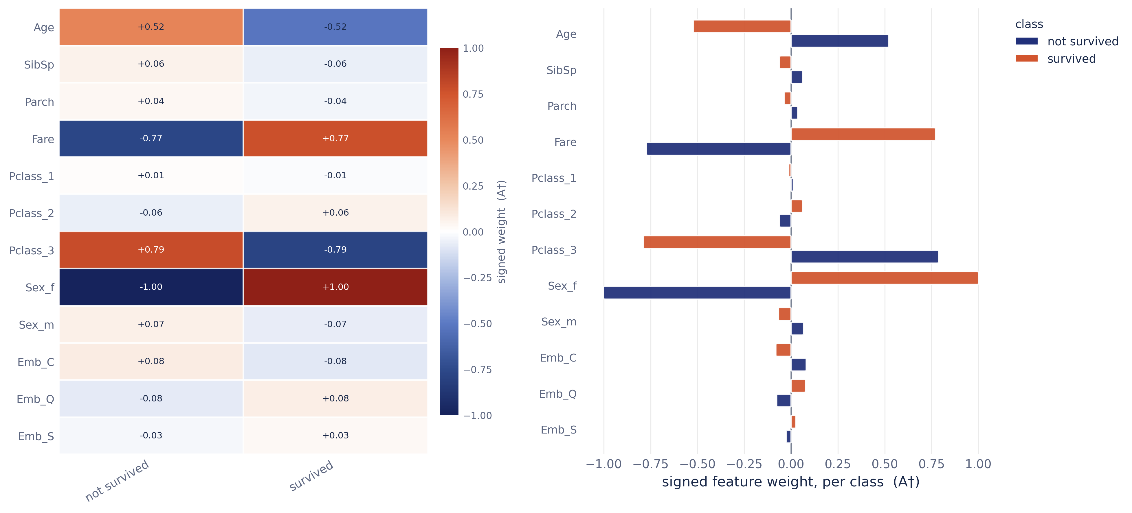
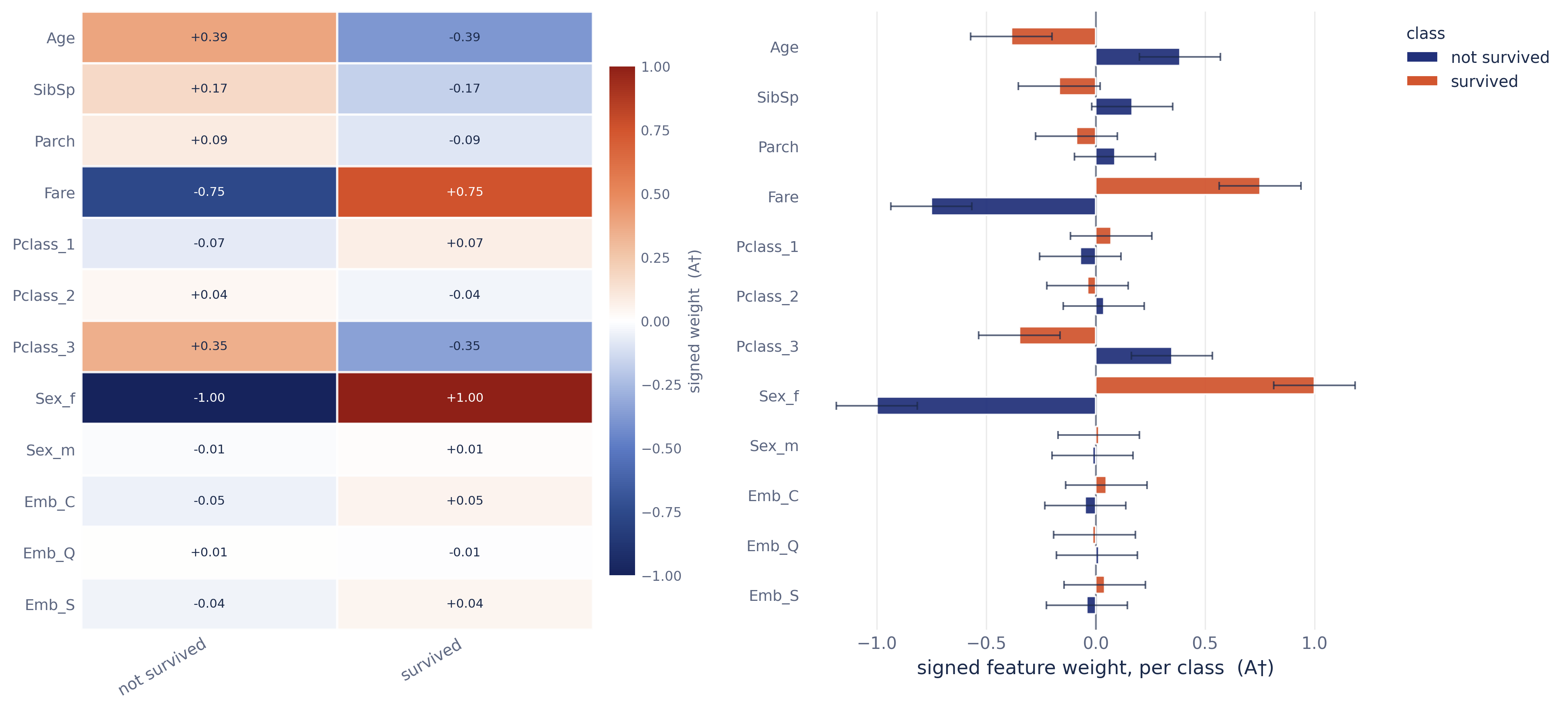
The left panel is the operator field (the signed A† matrix); the right panel shows per-class signed weights with a class legend — AIME's signature ability to give a distinct importance vector for every output class.

Local feature importance — one instance

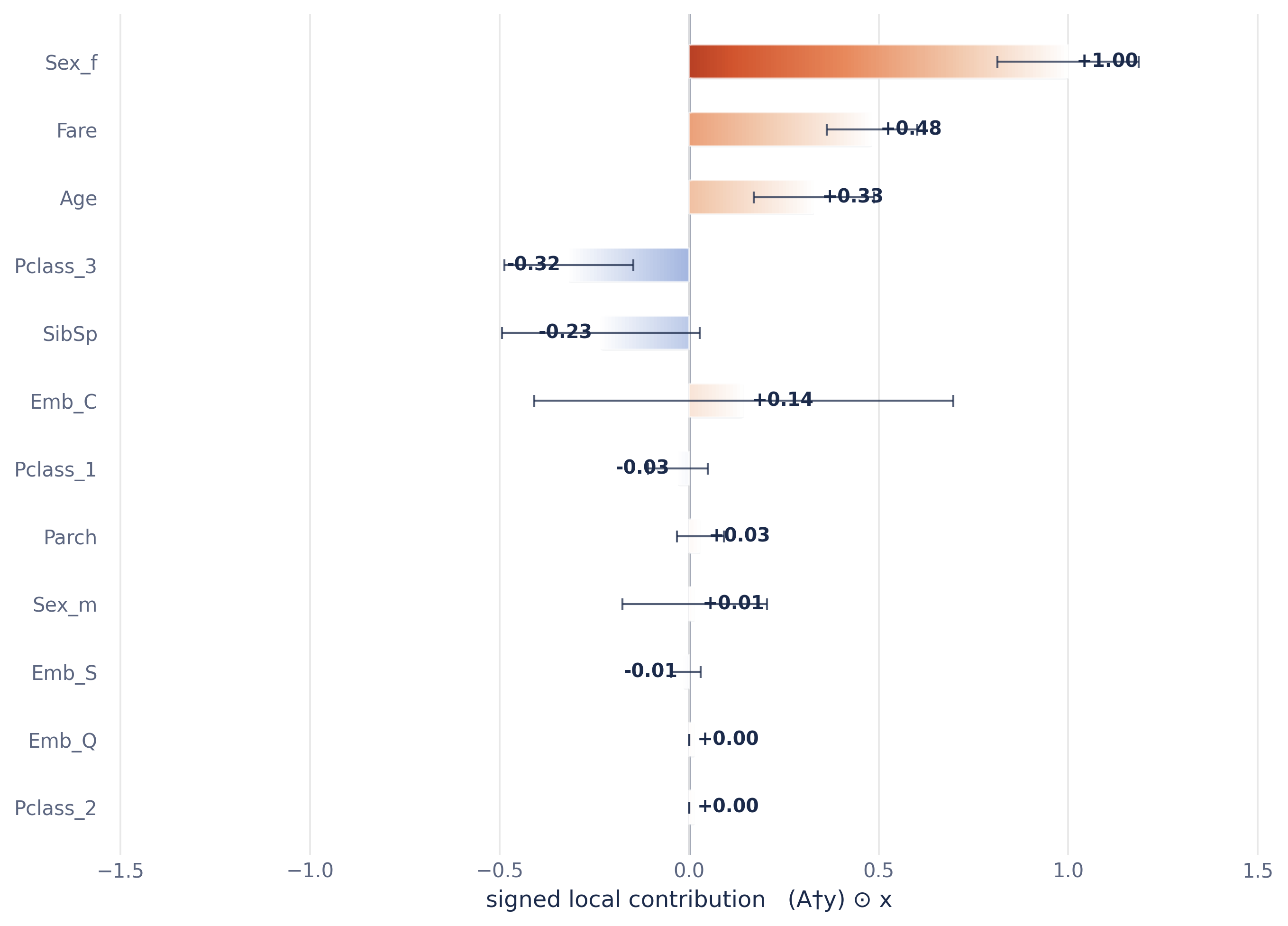
Local importance is the Hadamard product (A† y) ⊙ x'. Because it multiplies by the instance, features that are zero in x get exactly zero importance.

explainer.local_feature_importance(
    jack, [0, 1], feature_names=feature_names, scaler=explainer.scaler,
    ignore_zero_features=True, top_k=5).round(2)

   Sex_female  Fare  Pclass_3  Embarked_Q  Embarked_S
0         1.0  0.82     -0.79        0.05        0.02

---

Visualisation catalogue

Unique to the inverse-operator view (no LIME/SHAP equivalent)

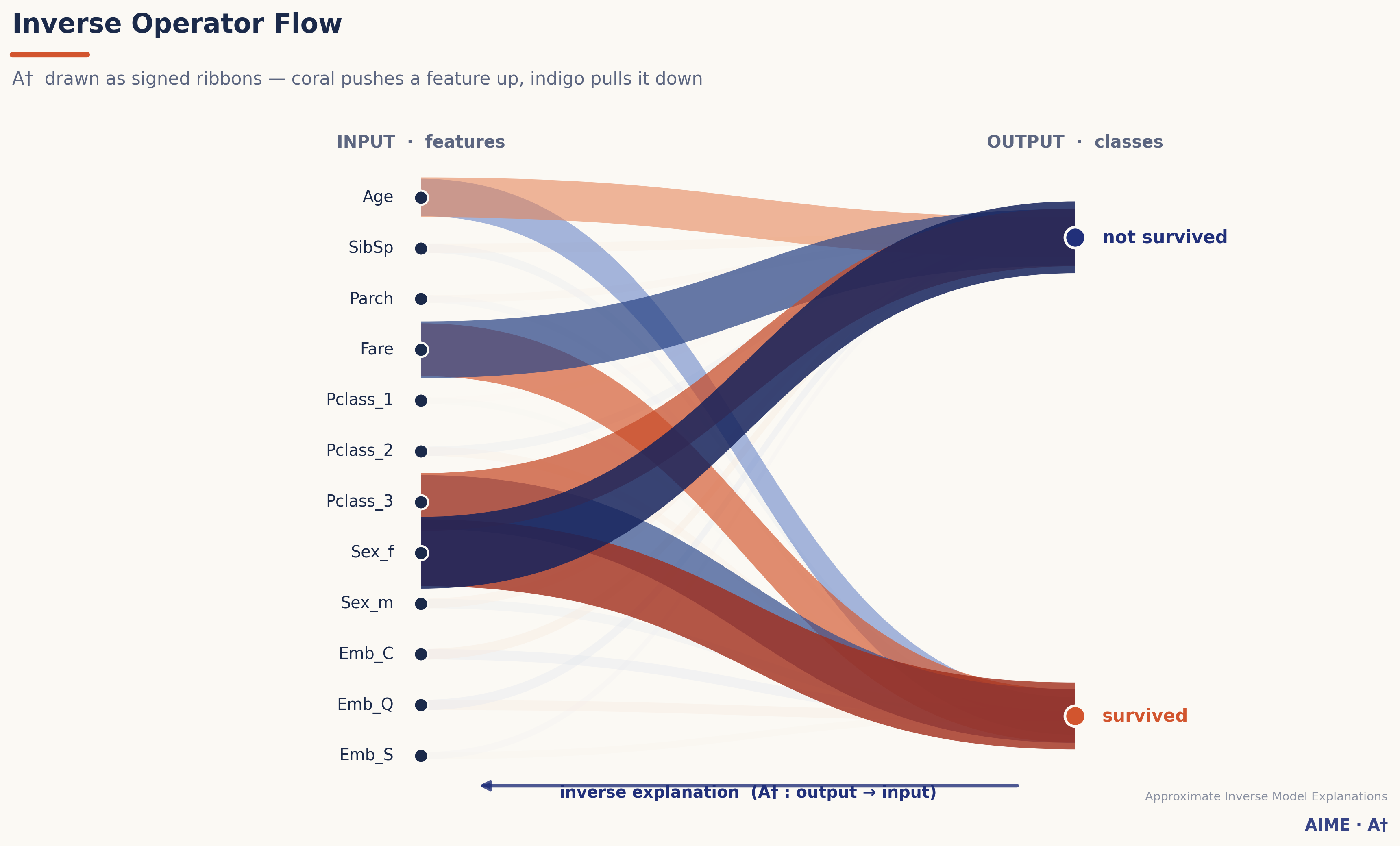
Inverse Operator Flow — A† itself, drawn as signed ribbons flowing output → input (the inverse direction). Coral pushes a feature up, indigo pulls it down; width = |weight|.

explainer.plot_inverse_operator_flow(feature_names=feature_names, class_names=class_names)

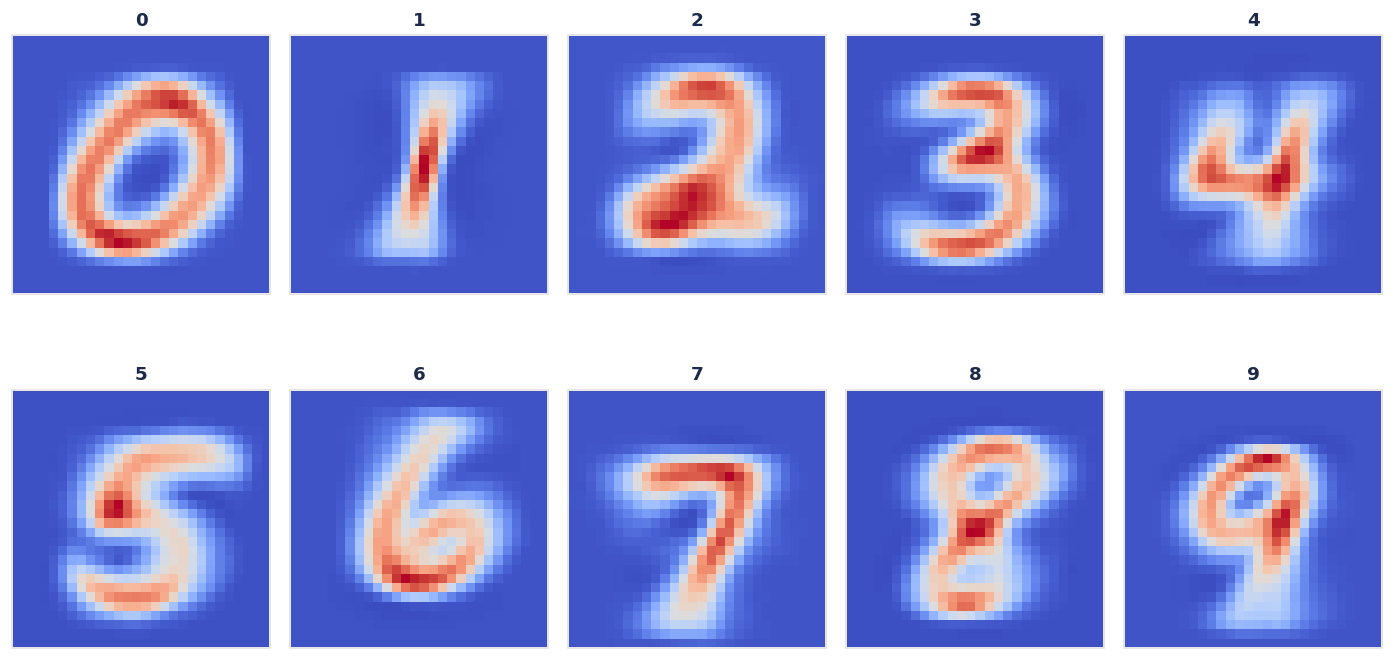
Representative estimation instances — A† eₜ, the ideal input the model reconstructs for each class. For image models it reconstructs an ideal class image; for tabular data, a feature fingerprint.

rep = explainer.representative_instance(scaler=explainer.scaler,
                                        feature_names=feature_names, class_names=class_names)
explainer.plot_representative_instance(scaler=explainer.scaler, image_shape=(28, 28))  # image models

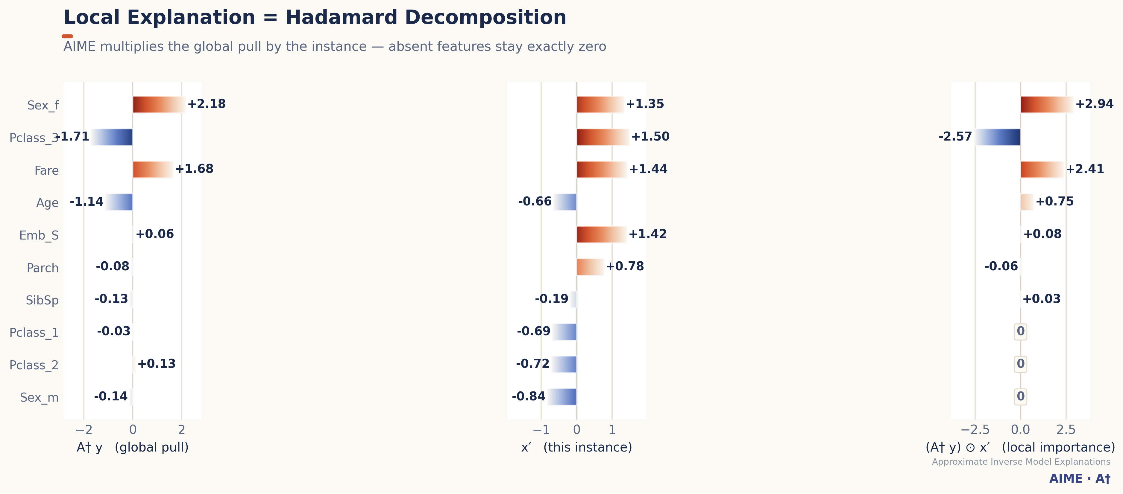
Local Hadamard decomposition — shows a local explanation being built as global pull × instance; absent features visibly collapse to exactly zero.

explainer.plot_local_hadamard_decomposition(jack, np.array([0., 1.]),
                                             feature_names=feature_names, top_k=12)

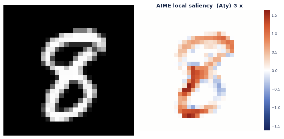
Local saliency (image models) — analytic saliency (A† y) ⊙ x reshaped onto the image grid. No gradients, no perturbations.

explainer.plot_local_saliency(x, y, image_shape=(28, 28), scaler=explainer.scaler)

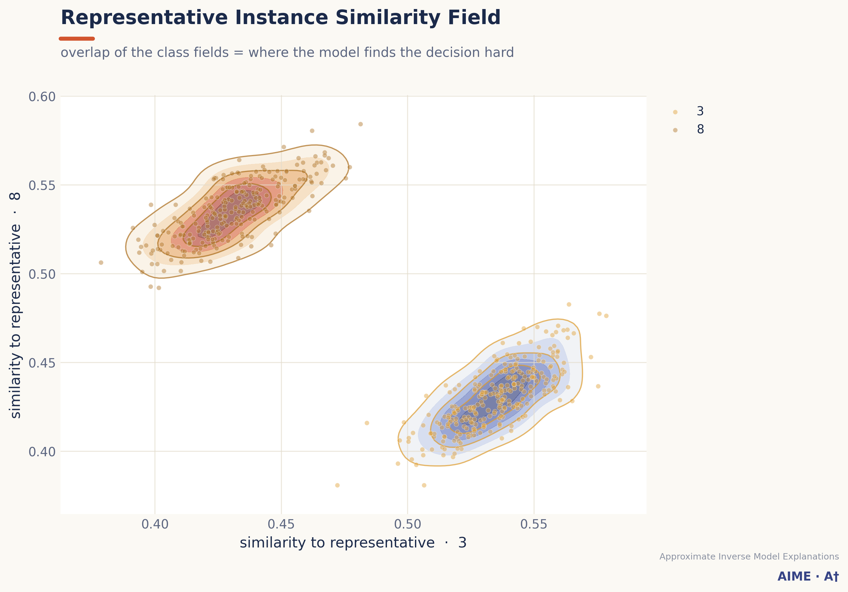
Representative instance similarity field — every point scored by RBF similarity to two classes' representative instances; the overlap is where the model finds the decision hard. Use gamma='scale' for high-dimensional inputs.

explainer.plot_rep_instance_similarity(
    X_test, y_hat_test, feature_names=feature_names, class_names=class_names,
    gamma='scale', class_indices=[3, 8])

---

BayesianAIME — uncertainty on the explanation

BayesianAIME estimates a posterior over A†, so the importance plots carry 95% credible intervals and the returned frames hold mean / lower_bound / upper_bound.

bayes = AIME(use_bayesian=True, bayesian_sigma=1.0, bayesian_tau=1.0)
bayes.create_explainer(X_train, y_hat_train, normalize=True)

bayes.local_feature_importance(jack, [0, 1], feature_names=feature_names, top_k=4).round(2)

             Sex_female  Fare  Pclass_3  Embarked_Q
mean               1.00  0.82     -0.79        0.05
lower_bound        0.89  0.71     -0.90       -0.06
upper_bound        1.11  0.94     -0.67        0.16

---

Note on RidgeAIME effectiveness

Whether RidgeAIME visibly differs from AIME depends on the data:

1. λ vs sample size. Ridge's λI competes with YᵀY, whose eigenvalues scale with N. On Titanic (N≈700) they are ~10²–10³, so the default λ=1e-3 changes the raw operator by only ~1e-5. Ridge becomes active once λ reaches that band.
2. Binary + normalisation. With two classes, Ridge rescales each class column of A† by an almost-constant factor, and the per-class peak normalisation in global_feature_importance divides it out — so even a large λ leaves the normalised importance essentially unchanged (for ≥3 classes the cancellation is only partial).

To judge Ridge, compare the raw operator A_dagger (or sweep λ):

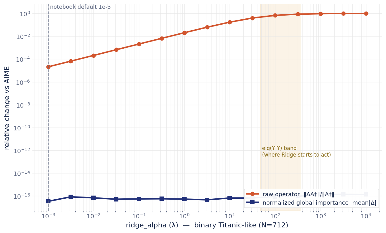
(raw-operator change rises with λ toward the eig(YᵀY) band; the normalised global importance stays at machine-zero for binary tasks.)

Publication mode (default on)

Figures are publication-clean by default: white background, no title/subtitle headers, no brand mark — only in-figure captions (axis labels, legends, value labels, colorbars), so a figure drops straight into a paper. To restore the titled/branded look (e.g. for slides):

import aime_xai.style as S
S.set_publication_mode(False)

---

Interactive explorers (render inline in Colab)

Both return a Colab/Jupyter object that displays inline when it is the last expression in a cell; pass path=... to also save a standalone .html.

explainer.interactive_operator_flow(feature_names=feature_names, class_names=class_names)

# set a target output y with sliders → reconstruct the input x = scaler⁻¹(A†·y) live.
# image models morph an ideal-image canvas; tabular shows a standardized z = A†·y profile.
explainer.interactive_reconstruction(image_shape=(28, 28), class_names=class_names,
                                     path='aime_reconstruction.html')

---

Preserved API

All public class/method names and signatures match the canonical implementation, so existing code keeps working; plotting methods only gain optional save_path / show arguments.

AIME(...) · create_explainer · global_feature_importance · global_feature_importance_each · global_feature_importance_without_viz · local_feature_importance · local_feature_importance_without_viz · representative_instance · plot_representative_instance · plot_inverse_operator_flow · plot_local_hadamard_decomposition · plot_local_saliency · rbf_kernel · plot_rep_instance_similarity · interactive_operator_flow · interactive_reconstruction · export_interactive

---

License

AIME is dual-licensed under the 2-Clause BSD License and a Commercial License. Apply the 2-Clause BSD License only for academic or research purposes, and the Commercial License for commercial and other purposes — you choose which to use. For commercial licensing (a fee may apply), contact takafumi@eigenbeats.com.

---

Citation

If you use this software, please cite the relevant paper(s).

@ARTICLE{10247033,
  author={Nakanishi, Takafumi},
  journal={IEEE Access},
  title={Approximate Inverse Model Explanations (AIME): Unveiling Local and Global Insights in Machine Learning Models},
  year={2023}, volume={11}, pages={101020-101044},
  doi={10.1109/ACCESS.2023.3314336}}

@ARTICLE{10979913,
  author={Nakanishi, Takafumi},
  journal={IEEE Access},
  title={HuberAIME: A Robust Approach to Explainable AI in the Presence of Outliers},
  year={2025}, volume={13}, pages={76796-76810},
  doi={10.1109/ACCESS.2025.3565279}}

@INPROCEEDINGS{IIAI-AAI-Winter2025-RidgeAIME,
  author={Itoh, T. and Nakanishi, Takafumi},
  booktitle={2025 19th IIAI International Congress on Advanced Applied Informatics (IIAI-AAI-Winter)},
  title={Approximate Inverse Model Explanations for Metamaterial Design with Scalar-Field-Based Metal Foam Surrogates},
  year={2025}, pages={179-184}, address={Phuket, Thailand},
  doi={10.1109/IIAI-AAI-Winter69777.2025.00041}}

@ARTICLE{BayesianAIME2025,
  author={Nakanishi, Takafumi},
  journal={IEEE Access},
  title={Bayesian-AIME: Quantifying Uncertainty and Enhancing Stability in Approximate Inverse Model Explanations},
  year={2025},
  doi={10.1109/ACCESS.2025.3617984}}

@ARTICLE{10648696,
  author={Nakanishi, Takafumi},
  journal={IEEE Access},
  title={PCAIME: Principal Component Analysis-Enhanced Approximate Inverse Model Explanations Through Dimensional Decomposition and Expansion},
  year={2024}, volume={12}, pages={121093-121113},
  doi={10.1109/ACCESS.2024.3450299}}

Author: Takafumi Nakanishi · takafumi@eigenbeats.com